Fractals: The Language of Nature, Art, and Math 

Author: Tri Le

Take a look at a square, a rectangle, or an equilateral triangle. Now think about something “natural” – originating from nature with minimum alterations made by humans. Can you come up with anything perfectly rectangular, a perfect 60-degree angle, or even a perfectly straight line in the wild? I don’t think so, and nor does a famous philosopher – Alan Watts. In his own words, using the notions of Taoism, an ancient Chinese philosophy about the Dao – the “way” or “course” of nature: 

The Dao is a certain kind of order, and this kind of order is not quite what we call order when we arrange everything geometrically in boxes or in rows. That is a very crude kind of order, but when you look at a bamboo plant, it is perfectly obvious that the plant has order. We recognize at once that it is not a mess, but it is not symmetrical and it is not geometrical. The plant looks like a Chinese drawing. The Chinese appreciated this kind of nonsymmetrical order so much that they put it into their painting. In the Chinese language this is called li, and the character for li originally meant the markings in jade. It also means the grain in wood and the fiber in muscle. We could say, too, that clouds have li, marble has li, the human body has li. We all recognize it, and the artist copies it whether he is a landscape painter, a portrait painter, an abstract painter, or a non-objective painter. They all are trying to express the essence of li. The interesting thing is that although we all know what it is, there is no way of defining it.

Alan W. Watts in Taoism: Way Beyond Seeking, The Edited Transcripts, ed. Mark Watts, Charles E. Tuttle Co., Boston, 1997.

Back in the early 1970s, this was quite true. Watts passed away in 1973, meaning that he missed a work achieving exactly what he considered difficult: finding the math to describe the geometry of nature. The work’s  name in English translation is “The Fractal Geometry of Nature” by none other than Benoit B. Mandelbrot (whose abbreviated B is humorously joked to stand for “Benoit B. Mandelbrot”)

Fractals, coined from the Latin word “fractus” meaning fragmented or irregular, are often thought of as shapes whose certain fragments are roughly a shrunken version of their entirety. But as their mind-boggling looks and diversity suggest, this is an oversimplification, and finding an umbrella mathematical definition for fractals is actually hard. For now, let’s stick with that common notion about self-similarity and check out some examples to grasp what they express.

Classical Examples in Math

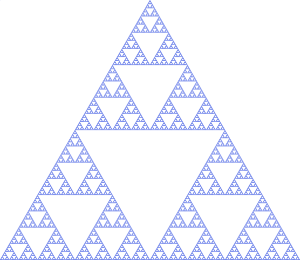
Start with an equilateral triangle and separate it into 4 equal smaller triangles. Remove the middle one then repeat this process for each newly formed equilateral triangle infinitely many times. The resulting shape is a Sierpinski triangle. 

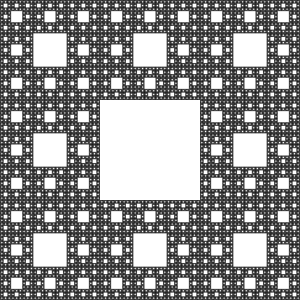
Replacing triangles with squares and dividing them into 9 instead of 4 squares in each step, we get what’s called a Sierpinski carpet. A similar fractal, made of segments instead of triangles, is the Cantor set: start with one colored segment, divide it into thirds, put copies of the first and third part right below them a small distance, and repeat indefinitely for each new segment.

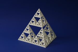
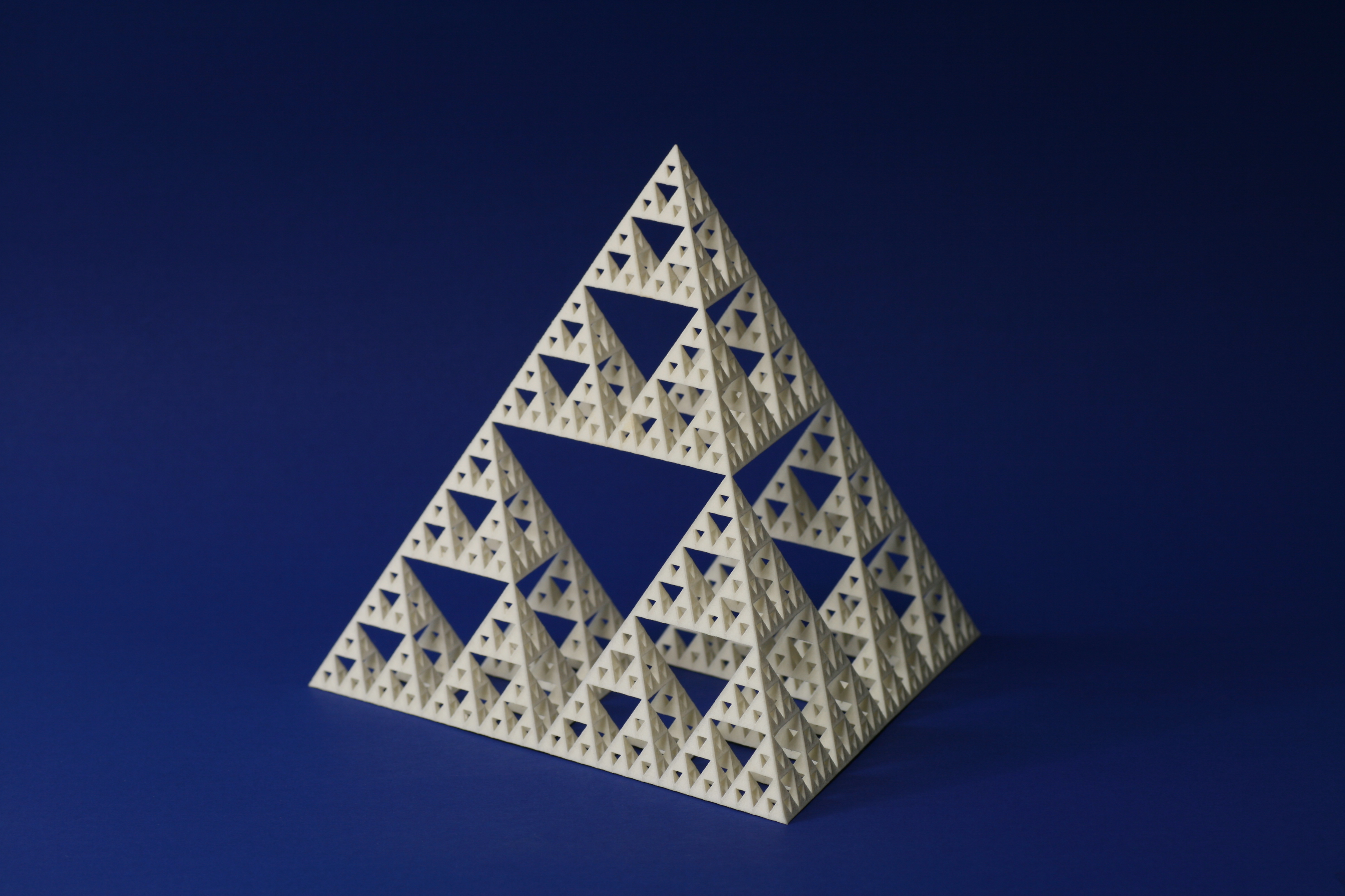
Of course, nothing’s stopping us from generalizing some of these structures: we can construct a fractal made of three-dimensional components instead of two: using regular tetrahedrons in place of equilateral triangles creates Sierpinski tetrahedrons while using cubes instead of squares results in a Menger sponge.

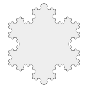
Another famous fractal is the Von Koch curve, built as follows:

From a starting line segment, divide it into 3 equal sections and construct an equilateral triangle pointing upward with the middle section as its side, then remove said middle section. Again, repeat this process for each segment created after each step infinitely many times.

Applying this procedure to the three sides of an equilateral triangle instead of a segment, you get a Von Koch snowflake.

By now I’m sure you have realized something in common with all of these fractals: we start with a certain shape and a sequence of geometrical changes applied to it infinitely many times. In more technical terms, we iterate a system of geometrical functions infinitely many times, which is why this fractal construction method the name “Iterated Function System” or IFS for short (Now you understand why the joke about Benoit B. Mandelbrot is funny). This is also one of the ways computers employ to render these impossible structures. 

This idea about repeating some procedure is also present in the generating method of other types of fractals, which will be briefly listed here:

• Strange attractors: they are attractors – a set of states that a dynamic system (such as differential or difference equations with varying initial conditions) tends to evolve into – with a fractal structure
• L-system: a recursive algorithm works according to several rules for replacing strings, the resulting strings after enough iterations are then turned into geometric structures. This method is useful in simulating branching patterns present in biology such as blood vessels and the shape of plants
• Escape-time fractals: are sets of points in space (such as the complex plane) satisfying the condition of some problem involving a formula or recursion relation applied to every point in space. Examples include the Mandelbrot set, along with Julia set, the Burning Ship fractal, and the Nova fractal. The name may come from the fact that applying the iteration to every point in space is significantly harder than iterating sufficiently many times on some individual mathematical object 
• Random fractals: formed by some stochastic rules
• Finite subdivision rules: tilings are refined by an algorithm involving continuous morphing (stretching, twisting, bending, etc), similar to the process of cell division.

Nature’s Language in the Form of Maths

The inherent ruggedness and complexity at any scale of fractals make them a great fit for describing the roughness of natural objects that the idealized Euclidean geometry fails to capture in full. Since it is impossible for humans to carry out “infinitely many” iterations, and atoms are not infinitely divisible, we can contend with a large-enough number of steps when attempting to create fractal images. We should be able to replicate the visual effects of a complete fractal since the added details will be virtually invisible. 

A pencil and paper should be useful in this section, as hands-on experience with this method of drawing is always more effective than reading only. Here are some examples:

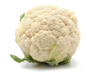
Cauliflower: Compare the floret and the entire cauliflower

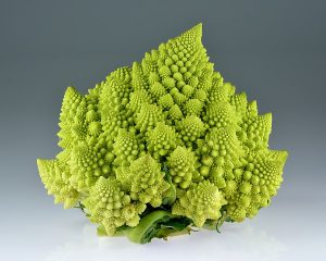
Romanesco Broccoli: notice how each bud is self-similar

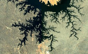
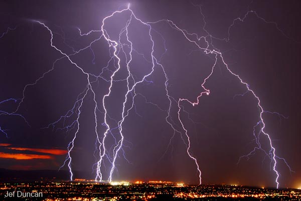
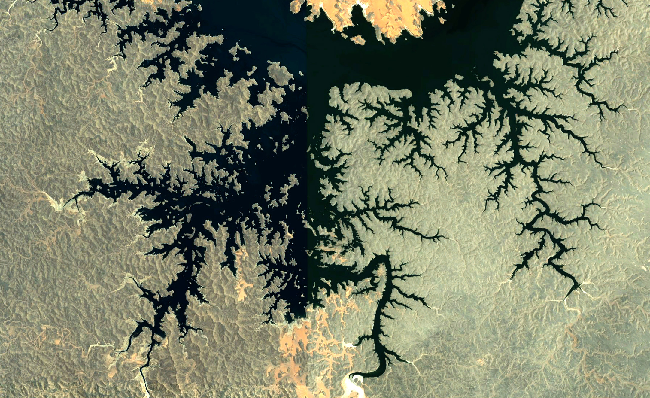
Mountain ranges also exhibit fractal structures. The featured image of this article was, in fact, rendered by fractal algorithms. Did you think it was real?

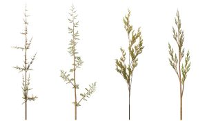
Try drawing something through the lens of fractals. First, use a sharp pencil to draw a tree branch that has no leaves, for example:

 Remember this shape, and replace each of the smaller branching sections with a shrunken version of this initial picture, and you may get something similar to this:

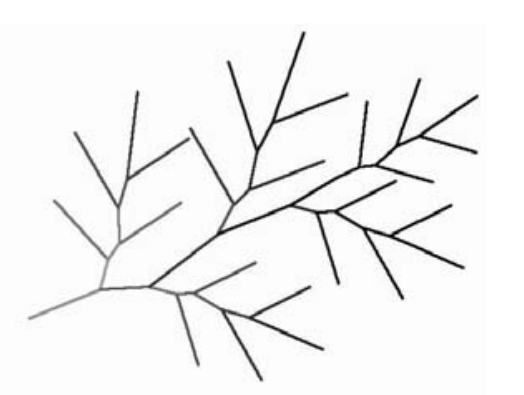
Not that close, but if you have the patience to do this a few times more, then either the tip of your pencil is not thin enough or you get 

This is applicable for other types of plants as well, depending on your initial drawing and the details you choose to iterate.

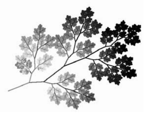
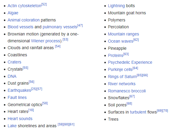
Here’s a more detailed list of where fractals appear in nature (you know where this picture is from):

Fractal Dimension: Math for Insight 

Of course, visually pleasing fractals aren’t beyond our reach or unable to be studied systematically. Expanding from our knowledge of conventional geometry, it is natural to attempt to implement existing concepts to fractals, starting with dimensions. As will be shown here, we need to rework this concept in a somewhat more unorthodox way.

In 1921, the British mathematician Lewis Fry Richardson, in one of his whimsical moments of applying Mathematics to unconventional subjects, tried tapping into the problem of measuring the length of coastlines

Richardson’s idea was to measure a coastline by choosing a “step size” s and then seeing how many steps it took to “walk” along the coast. For example, a walk goes from Land’s End to Duncansby Head, Richardson’s starting and ending points. When s = 100km it takes 28 steps to get to Duncansby Head, so Richardson would estimate the resulting length L to be 28s. This is illustrated in the first figure.

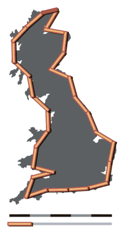
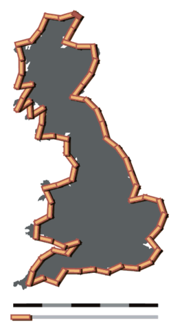
However, we see that such a large step size misses a lot of the detail of the coast—a lot of the “ins and outs”—so Richardson used successively smaller steps s and each time recorded the corresponding total length L. Instead of plotting L and s themselves, Richardson cleverly plotted their logarithms instead. At first, the coastline seems highly irregular and random—which is unlikely to have any simple mathematical pattern—the result was surprising: the data for the coast of Britain and several other countries formed convincing straight lines!

Each line has an equation of the form: log L = m log s + b. (here log is base 10)

Using Richardson’s original data we find that the line associated with the length in kilometers of the west coast of Britain roughly satisfies the equation:

log L = -0.25 log s + 3.7.

which when we take the exponent of both sides gives us:

L ≈ 5000/(s^0.25)

But this means that the smaller we reduce the step size s the larger L becomes without bound. Since coastlines are also considered fractals, this may suggest that all coastlines are in fact infinitely long! This feels somewhat sketchy, I’m sure you have seen some data on coastline length before, so the whole situation begs the question:

What did we do wrong?

How can we possibly measure a geometric object and get a result of infinity? Let’s repeat the process, by measuring the length of a square. Not just the perimeter, but the entire interior as well. 

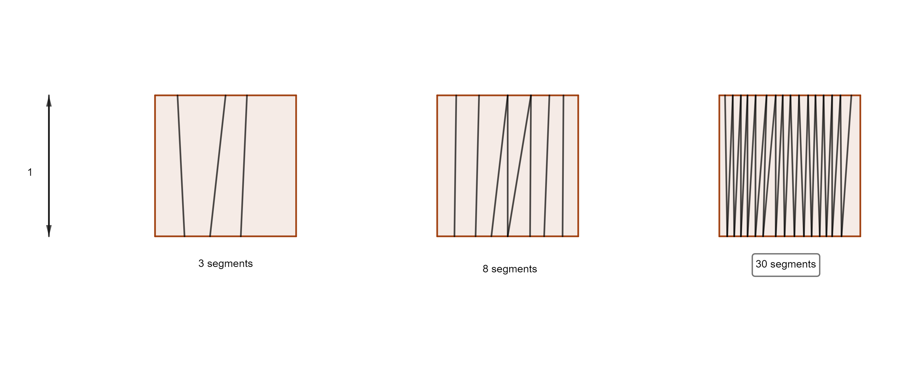
But how many segments do we need to fit the square’s interior? No matter how many, even when the segments are so tightly packed that the pixels on the screen cannot display that amount of detail, it’s still not enough to fit the entirety of the square. We can go on forever and there will still be gaps between any different segments. So we conclude that the square is infinite in length.

How about measuring the volume of the square? Clearly 0, since a square has a width and length, but no thickness. After all the shenanigans, what’s the takeaway lesson?

We’re measuring it the wrong way. In the wrong dimension that is. 

A square should be measured in 2-D, which is its area. But our coastline is a rugged line, so it cannot have an area. Yet it’s infinite in length, so how can it be one-dimensional? Maybe the answer is something in between? That is indeed the case here, before that, let’s return to our Euclidean shapes.

A segment has one dimension. Scaling it by a factor of 2 clearly makes its size 2^1 = 2 times the original size.

Scaling a square, which is 2-dimensional, gives us a square of area 2^2 = 4 times our starting square.

As for a cube, when a side is doubled, its volume goes up by a factor of 2^3 = 8, and 3 is also the dimension of this object.

This procedure is feasible even for the coastline. We’ve already intuitively established that the dimension of the segment is not enough for measuring this rugged boundary. That’s why we use squares instead, utilizing their larger dimension. 

Imagine that you put a map of Britain on a square grid, and count the number of unit squares that the coastline intersects. Then, use a grid with squares half the side length of the grid we’ve just used and count the intersected unit squares once more. In the same vein of logic as before, the dimension d of the coastline should satisfy:

2^d = the number of unit squares of the latter map/ that of the former map

If we do this for more and more detailed grids, meaning that the squares’ side lengths shrink, the value on the right-hand side will become closer and closer to some number, which when we take the logarithm in base 2 of both sides is the value of d. For the British coastline, d is approximately 1.21, which is indeed between 1 and 2 as we expected.